Skip to content
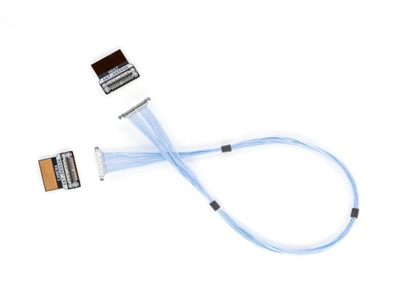
A micro coax assembly can look almost perfect on a drawing and still behave very differently once a multi-gigabit signal starts moving through it. Two tiny coax lines may leave the same connector, follow the same route and finish at the same nominal length, yet a small difference in dielectric geometry, conductor position, shield opening or connector termination can make one side of the differential channel arrive earlier or reflect more energy than the other. That is the practical reason pair matching deserves attention: at high speed, visual symmetry is not the same as electrical symmetry.
Micro coax pair matching is the control of electrical similarity between the P and N paths of a differential channel. It includes physical length, electrical length, propagation delay, impedance behavior and termination geometry. Good matching limits intra-pair skew, helps preserve differential-mode energy, reduces unnecessary common-mode conversion and protects timing margin at the receiver. Equal cut length is useful, but it is only one part of the finished-channel requirement.
The issue becomes easier to appreciate when the timing is converted into familiar numbers. At 10 Gbps NRZ, one bit period is only 100 ps. A published micro-coax study from I-PEX reported about 3.5 ps of effective intra-pair skew with a 1 mm intentional P/N mismatch and about 16.6 ps with a 4 mm mismatch under its stated 10 Gbps simulation conditions. Those figures are not universal acceptance limits, but they show how a dimension that seems trivial on the workbench can consume meaningful timing margin inside a fast link.

What Is Micro Coax Pair Matching?
Micro coax pair matching means keeping the two signal paths of a differential channel electrically similar enough to satisfy the interface’s signal-integrity limits. The matching target can include physical length, electrical length, propagation delay, impedance and termination symmetry. It is broader than simple length matching because two cables that measure the same in millimeters can still produce different delay, reflection or connector-transition behavior.
| Matching Item | Practical Measurement | Main Risk if Mismatched |
| Physical length | mm | Basic path-delay difference |
| Propagation delay | ps or ps/m | Intra-pair skew |
| Single-ended impedance | ohms | P/N electrical imbalance |
| Differential impedance | ohms | Reflection and eye degradation |
| Termination geometry | mm / controlled dimensions | Local discontinuity |
| Shield / return transition | structure + continuity | Mode conversion and EMI |
| Connector transition | TDR / VNA response | Reflection and delay asymmetry |
What Is Actually Being Matched?
A high-speed differential receiver responds to the difference between the positive and negative signals, so the two paths need to behave as a coordinated pair rather than as unrelated wires. In a micro coax assembly, that balance can be influenced by cable length, propagation velocity, local impedance, conductor geometry, shield geometry and the way each line transitions into the connector. The finished assembly is therefore the relevant object to judge. A raw cable datasheet may confirm a nominal impedance or propagation characteristic, but it does not automatically describe what happens after stripping, soldering, grounding and routing have been added.
The word matching can also create confusion because different specifications use it in different ways. Some standards use pair matching narrowly for the impedance relationship between the two single-ended paths, while engineers in everyday high-speed development may use the same phrase more broadly when discussing delay, skew and overall P/N symmetry. During an RFQ or design review, the useful question is not simply whether the pair is matched. The useful question is which parameter must match, what tolerance applies, where the measurement reference planes sit and which test proves compliance.
Length Matching vs Electrical Matching
Physical length is the easiest matching parameter to put on a drawing because it can be measured directly in millimeters. Electrical length is different: it represents the time or phase behavior of the transmission path, so it depends on both physical distance and propagation velocity. Two 150 mm lines can therefore have slightly different electrical lengths if their dielectric structure, conductor geometry or termination exposure is not identical. At high data rates, engineers increasingly care about the resulting delay in picoseconds because that is what the receiver experiences, even though manufacturing still needs mechanical dimensions to control the process.
This distinction prevents a common mistake: assuming that a strict cutting tolerance guarantees high-speed performance. Cutting accuracy removes one major source of mismatch, but the connector launch, exposed center conductor, shield fold-back, local cable compression and PCB transition can add electrical asymmetry after the cut is complete. A sensible design links mechanical dimensions to an electrical target. Overall length may be controlled for fit, while a tighter relative P/N tolerance, strip-length control and defined termination geometry protect the signal. For demanding links, TDR or delay measurements then confirm whether the physical process actually delivered the expected electrical result.
Intra-Pair vs Pair-to-Pair Matching
Intra-pair matching compares P with N inside one differential channel. If one side arrives later, the difference is intra-pair skew, and the differential waveform itself becomes less balanced. Pair-to-pair or lane-to-lane matching compares one complete differential channel with another. That can matter in multi-lane interfaces, but it is a separate problem: a cable can have excellent P/N matching within every lane and still have noticeable timing differences from Lane 1 to Lane 4, or it can have closely aligned lanes while one lane contains poor P/N balance.
This distinction becomes especially important in dense micro coax assemblies where dozens of signal paths share one fine-pitch connector. A 40-channel harness may include several differential data lanes, clock pairs, grounds, control lines and power conductors. The drawing should preserve pair identity, polarity and lane assignment instead of treating all positions as independent point-to-point wires. Continuity testing can confirm that each pin reaches the expected destination, but it may not reveal a broken pair architecture if the test program does not understand which pins belong together. Pair mapping is therefore part of signal-integrity control, not just documentation.

Which Parameters Determine Pair Matching?
Pair matching is mainly determined by propagation delay, impedance consistency, cable geometry, dielectric properties and connector termination. The finished assembly matters more than the raw cable alone because stripping, soldering, shield opening, pin transitions and mechanical deformation can change P and N after otherwise well-controlled micro coax leaves the spool. A robust design therefore controls both cable construction and assembly geometry.
Impedance and Pair Balance
Characteristic impedance is one of the first parameters engineers review because high-speed signals behave as traveling waves. Many common differential links use nominal targets around 90 ohms or 100 ohms, while the exact value and tolerance must follow the interface, PCB design and customer specification. It is also important to distinguish a nominal differential number from actual pair balance. A simplified 100-ohm description does not prove that P and N are behaving equally if one side contains a stronger local discontinuity, a different transition or a larger reflection than the other side.
Assembly-level control is therefore more informative than relying only on the cable datasheet. The raw cable may be manufactured to a controlled impedance, but the electrical environment changes where the coax shield is opened and the signal enters a connector contact, solder pad or PCB launch. Unequal strip lengths, excessive solder, different shield fold-back, conductor movement or connector seating can create local capacitance and inductance differences. In a serious design review, the acceptance definition should identify whether the connector is included, where the reference plane is located, what tolerance is allowed and whether local discontinuities are judged separately from the nominal cable body.
Propagation Delay and Dielectric
Propagation delay is the time a signal takes to travel through the cable, and it is governed by both physical length and propagation velocity. Propagation velocity depends heavily on the dielectric environment around the conductor, which means AWG alone cannot tell an engineer how fast a signal will travel. Two miniature coax products with the same conductor gauge can still have different capacitance, dielectric constant, velocity factor, shielding construction and insertion loss. For pair matching, consistency between P and N is often more important than whether the absolute delay is slightly higher or lower than another cable family.
Dielectric geometry deserves particular attention in micro coax because the dimensions are small and mechanical disturbance can alter the local electromagnetic structure. Conductor concentricity, dielectric diameter, cable compression during bundling, tight ties and excessive bending can all shift impedance or delay to some degree. Temperature can also influence material dimensions and electrical properties, although the practical importance depends on the application. A stable cable construction, controlled supplier and frozen BOM usually provide more value than attempting to calculate every microscopic variable. When performance margin is tight, the final assembly should be characterized rather than assumed to behave exactly like an ideal cable model.
Connector and Termination Geometry
The connector is often the most difficult part of the channel to keep symmetrical because controlled coax geometry must eventually be opened. The shield stops, dielectric is exposed, the center conductor enters a terminal or solder region and the return path changes shape. If the P side has 1.0 mm of exposed conductor while the N side has 1.8 mm, the transition is no longer electrically identical even if the cable bodies are perfectly matched. Similar effects can come from uneven shield termination, solder volume, pin length or connector-ground geometry.
A practical review therefore looks beyond the cable body and asks where controlled geometry ends, how long the exposed signal path is, where the return current flows, whether P and N are terminated in the same way and whether the connector launch introduces a visible disturbance on TDR or frequency-domain measurements. This is also why changing to a mechanically compatible connector can require new high-speed validation. The new part may mate correctly and pass continuity while presenting a different internal pin field, ground arrangement or launch geometry that changes reflection, delay or common-mode behavior.
Do Both Micro Coax Lines Need the Same Length?
The two micro coax lines should normally be closely matched, but identical physical length is not the final requirement. The real target is keeping P and N within the electrical-delay and skew budget of the interface. Physical length control is a practical manufacturing method; electrical matching is the performance goal. The acceptable tolerance depends on data rate, cable velocity, connector transition and available channel margin.
| P/N Length Difference | Approx. Delay Difference at VF 0.65-0.80 | Share of 100 ps UI at 10 Gbps |
| 0.5 mm | 2.1-2.6 ps | 2.1-2.6% |
| 1.0 mm | 4.2-5.1 ps | 4.2-5.1% |
| 2.0 mm | 8.3-10.3 ps | 8.3-10.3% |
| 5.0 mm | 20.9-25.7 ps | 20.9-25.7% |
Physical Length Is Only a Proxy
Engineers specify length because it is easy to measure and reproduce, but millimeters do not convert into picoseconds until propagation velocity is known. For a rough engineering estimate, a cable with a velocity factor between 0.65 and 0.80 has about 5.1 to 4.2 ps of delay per millimeter. Actual micro coax must use the cable manufacturer’s data or measurement, yet the estimate is enough to show why a one-millimeter difference can matter in a fast link. The signal responds to absolute time difference, not to the percentage of total cable length represented by that millimeter.
The same logic applies to short assemblies. A one-millimeter mismatch in a 300 mm cable may sound like only 0.33% mechanically, but it can still represent several picoseconds of timing difference. At 10 Gbps NRZ, one bit period is 100 ps, so a few picoseconds can consume a visible portion of the unit interval. That does not mean every system fails at that point; receiver margin, equalization, jitter, PCB routing and connector performance all matter. It simply means that the relevant engineering conversation should be about skew budget rather than percentage-of-length alone.
How Tight Should Matching Be?
There is no responsible universal rule that every micro coax differential pair must be matched within 0.5 mm, 1 mm or any other single value. The tolerance has to come from the electrical requirement. At 5 Gbps NRZ, one bit period is 200 ps; at 10 Gbps it is 100 ps; at 20 Gbps it is 50 ps. The same 5 ps cable-induced skew therefore occupies a progressively larger fraction of the timing window as data rate rises, especially when other channel impairments have already consumed part of the margin.
The strongest workflow is to start with the interface and allowable skew, then work backward into cable construction and manufacturing dimensions. If the complete channel allocates only a few picoseconds to cable-induced mismatch, the process may need tight relative P/N cutting, controlled strip dimensions, stable raw material and electrical verification. If the system has generous margin, forcing extremely tight mechanical tolerances can add cost without creating meaningful benefit. Good engineering avoids both extremes: loose tolerances that do not protect performance and unnecessarily tight tolerances that make production fragile or expensive.
Electrical Length Can Matter More
Two lines can both measure 150.0 mm and still exhibit different electrical delay if their terminations or dielectric environments are not identical. One side may have more exposed conductor, a longer unshielded transition or a different path through the connector. Another side may be compressed near an overmold or routed through a tighter bend. In those cases, the ruler says the pair is matched while the signal sees two slightly different transmission paths. That is the point at which electrical-length or delay measurement becomes more useful than relying only on finished mechanical dimensions.
Electrical matching also matters during material substitution. A new 50 AWG micro coax may fit the same space and have the same outside diameter as the approved cable, yet its dielectric construction and propagation characteristics can differ. If the project depends on a tightly managed skew budget, the replacement should be treated as an engineering change and validated accordingly. This is a practical reason to freeze approved cable part numbers in the BOM for high-speed assemblies instead of allowing purchasing teams to swap visually similar materials without checking the resulting channel behavior.

How Does Pair Mismatch Affect Signal Integrity?
Pair mismatch makes P and N behave less like a balanced differential channel. The most direct result is intra-pair skew, but the effects can extend to common-mode conversion, EMI, reduced eye opening and lower receiver timing margin. A small mismatch may be harmless in a robust link, while the same mismatch can become important when loss, reflection, jitter or crosstalk have already consumed channel margin.
Skew and Timing Margin
An ideal differential transmitter launches complementary P and N transitions that reach the receiver at nearly the same time. If one path is electrically longer or slower, one transition arrives later and creates intra-pair skew. At 10 Gbps NRZ, a 10 ps P/N difference occupies 10% of a 100 ps unit interval. At 20 Gbps, the same 10 ps occupies 20% of a 50 ps unit interval. Those percentages do not directly predict pass or fail, but they make the shrinking timing window easy to understand.
Skew also interacts with impairments that are already present elsewhere in the channel. Transmitter jitter, PCB trace mismatch, connector reflection, insertion loss, crosstalk and receiver uncertainty can all consume timing or voltage margin. The cable does not need to be the largest contributor to become relevant; it only needs to push a marginal system past the point where equalization or sampling can no longer recover the signal reliably. That is why a cable that works comfortably at one data rate or length can become unstable after a bandwidth increase, longer route or connector change.
Mode Conversion and EMI
Differential signaling is attractive partly because equal and opposite currents tend to cancel external fields. When the two sides are no longer well balanced in timing or amplitude, that cancellation becomes less effective and some intended differential energy can convert into common-mode energy. Common-mode current is more likely to interact with connector shells, cable shields, chassis structures and nearby conductors, which can increase radiated emissions or make the link more sensitive to environmental noise. Published micro-coax work from I-PEX has demonstrated increasing differential-to-common-mode conversion as intentional P/N mismatch grows under its stated test conditions.
This is also why shielding and pair matching should not be treated as interchangeable fixes. A strong shield can help contain fields and provide a controlled return environment, but it does not remove the underlying delay imbalance between P and N. Conversely, excellent pair matching does not compensate for a shield that is badly terminated or a return path that breaks at the connector. When EMI appears after a cable change, an experienced investigation reviews pair geometry, skew, shield continuity, connector grounding, PCB return path and routing together instead of tightening one mechanical tolerance and assuming the problem is solved.
Eye Margin and Link Stability
An eye diagram combines many repetitions of the transmitted data waveform, so it is useful for seeing the total effect of channel impairments. A wide open eye indicates useful timing and voltage margin, while skew can contribute to horizontal closure or shifted zero crossings because the P and N edges no longer reinforce the differential transition at exactly the same moment. If one side of the pair also experiences a stronger reflection, the receiver may see timing asymmetry and amplitude distortion together rather than a clean single impairment.
In real equipment, the symptoms can be less tidy than the laboratory plot. A camera link may show occasional frame loss, a display may flicker only at a particular resolution, or an embedded system may retrain the link after the cable is bent into its installed position. Those symptoms do not prove pair mismatch, because contact resistance, power integrity, insertion loss, software and other causes can look similar. The reliable troubleshooting sequence is to reproduce the failure, measure the relevant channel parameters, localize the disturbance, change one variable and verify the result under the same conditions.
How Is Micro Coax Pair Matching Tested?
Micro coax pair matching is usually evaluated with time-domain and frequency-domain measurements. TDR can reveal impedance profiles, discontinuities, propagation delay and skew, while a VNA can show insertion loss, return loss and mixed-mode behavior versus frequency. Eye-diagram, BER or system-level tests may then confirm application performance when cable-level measurements alone are not enough to prove the required high-speed operating margin.
| Test | Typical Output | What It Helps Diagnose |
| TDR | ohms vs time / distance | Impedance profile and discontinuity location |
| Propagation delay | ps or ns | Electrical length mismatch |
| Intra-pair skew | ps | P/N timing difference |
| VNA insertion loss | dB vs frequency | Channel attenuation |
| VNA return loss | dB vs frequency | Reflections |
| Mixed-mode S-parameters | dB vs frequency | Differential/common-mode conversion |
| Eye diagram | voltage / time opening | Combined timing and voltage margin |
| BER / system test | error rate / functional result | Application-level performance |
TDR and Differential TDR
Time-domain reflectometry is one of the most useful tools for high-speed cable development because it shows where an impedance event occurs along the signal path. A fast edge is launched into the assembly and the reflected energy is displayed against time, allowing engineers to distinguish the connector transition from the cable body and far-end termination. For a micro coax pair, the two sides can be compared individually or in a differential measurement to examine local impedance, propagation delay, connector discontinuity and relative P/N behavior.
The fixture is part of the measurement and can easily create misleading results if it is not controlled. If the two test paths differ by several picoseconds, the instrument may report apparent skew that belongs to the fixture rather than the device under test. Proper calibration, de-skewing, reference-plane definition and repeatable fixturing are therefore essential. A meaningful report should state the test setup and acceptance region instead of presenting a single impedance number without context. This becomes especially important when a customer wants to compare prototypes from different suppliers or different cable revisions.
VNA and Mixed-Mode Measurements
A vector network analyzer evaluates the assembly in the frequency domain and becomes valuable when engineers need to understand how the channel behaves across the bandwidth of the actual signal. Insertion loss shows how much signal energy is attenuated, return loss describes reflection, and mixed-mode S-parameters can reveal how differential energy converts into common mode. That last measurement is particularly useful when pair imbalance is suspected because a cable can pass continuity and still create undesirable high-frequency mode conversion.
The measurement bandwidth should be tied to the real interface rather than chosen simply because the instrument can sweep to a higher frequency. A test that ends too low may miss the behavior that matters to a multi-gigabit edge, while testing far beyond the useful bandwidth can add cost and produce data that does not change the engineering decision. The acceptance plan should therefore define the protocol or relevant frequency range, fixture, reference planes and the specific S-parameters that matter. This keeps validation focused on the failure mechanisms the finished system actually needs to control.
Eye, BER and System Validation
Not every micro coax assembly needs an eye diagram or BER test. If the design uses a proven cable construction, generous margin and a well-understood connector system, continuity, pinout, dimensional inspection and the required impedance checks may be enough. More demanding links benefit from eye or BER testing when the combined effect of skew, insertion loss, reflection, crosstalk and jitter needs to be evaluated at the receiver. The decision should follow project risk rather than a marketing claim that every cable receives every possible high-frequency test.
System testing can be even more useful in camera, display and embedded applications because it proves the cable inside the environment where it will actually operate. A camera cable may be checked for stable image transfer and frame integrity; a display assembly may be exercised at the intended resolution and refresh rate; an embedded link may be tested through its normal boot, training and sustained-data conditions. Cable-level measurements explain the channel, while system validation answers the customer’s final question: does the approved assembly operate reliably in the real product under the defined installation conditions?
How Do Manufacturers Control Pair Matching?
Manufacturers control pair matching by translating electrical requirements into repeatable physical and process controls. Cable construction, relative P/N length, stripping, conductor exposure, connector termination, shield geometry, channel mapping and routing must be defined and maintained. Prototype data establishes the approved baseline, while controlled drawings, BOMs, fixtures, inspection, electrical testing and revision management keep later production close to the validated design.
Cable and Process Control
Pair matching starts with material control because an assembly cannot remain electrically repeatable if the raw cable construction changes without review. Two products can both be labeled 50 AWG and still have different dielectric structures, capacitance, propagation velocity or shielding performance. For a high-speed design, the BOM should identify the approved cable construction or manufacturer part number where those characteristics matter. Purchasing flexibility is valuable, but substitutions should be evaluated against the actual electrical requirements instead of approved only because the outside diameter and conductor gauge appear equivalent.
Production controls then focus on the dimensions that influence symmetry: relative P/N cut length, strip length, dielectric exposure, conductor condition, shield opening, connector seating and formed routing. The tightest tolerance is not always the overall finished length. A 250 mm cable may reasonably allow several millimeters of installation tolerance while the relative P/N cut difference or exposed conductor geometry needs much tighter control. This is the practical value of identifying signal-critical dimensions separately from ordinary fit dimensions: it directs tooling, operator attention and inspection effort toward the characteristics that actually protect high-speed performance.
Mapping, Polarity and Termination
High-density assemblies create another failure mode that has nothing to do with length: the wrong conductors can be paired or polarized incorrectly. A fine-pitch connector with dozens of positions may carry several data pairs, clock, grounds, controls and power. The production definition should preserve lane number, pair ID, P/N polarity, connector position and ground assignment from the engineering drawing through the work instruction and electrical test program. This makes it harder for a pair to be accidentally split during grouping or termination even when every individual wire still reaches a valid destination.
Termination needs the same discipline. Precision cutting can produce excellent relative cable length, yet inconsistent hand stripping can recreate electrical mismatch at the connector. Process engineers therefore watch strip-tool condition, center-conductor damage, exposed dielectric, conductor straightness, solder volume, terminal alignment and shield fold-back. Fine micro coax leaves little room for uncontrolled variation, so dedicated fixtures or positioning aids may provide more repeatability than relying on operator skill alone. A good manufacturing plan uses tooling to make the correct geometry easy to repeat and uses inspection or electrical data to catch drift before it becomes a shipment-level problem.
Prototype to Repeat Production
A prototype that passes once is useful evidence, but it is not yet a manufacturing capability. The stronger question is whether the electrical behavior can be reproduced across operators, material lots and repeat orders. The development record should therefore connect the requirement, controlled drawing, prototype, validation result and approved revision. Once the design is released, the BOM, work instruction, critical dimensions, test criteria and reference sample should all point back to the same approved baseline so production does not quietly drift away from the version the customer actually validated.
Change control is especially important for high-speed micro coax because apparently minor substitutions can alter the transmission path. A new connector may mate perfectly but present different launch geometry; a new cable may share AWG and OD but have a different propagation characteristic; a revised overmold may compress the cable differently near the termination. These changes should trigger an engineering review proportionate to the risk. For a new SINO-CONN development project, providing the interface, data rate, connector part number, pinout, cable length, target impedance, installation constraints and required validation method allows the engineering team to define pair matching in measurable terms before the design moves into repeat production.
Conclusion
Micro coax pair matching is best understood as a finished-channel discipline rather than a single dimension on a drawing. Physical length matters because it is one of the largest and easiest sources of delay mismatch to control, but electrical length, impedance, dielectric consistency, connector transition, shield geometry and production repeatability all influence what the receiver finally sees. The right tolerance therefore comes from the interface and signal-integrity budget, not from a universal millimeter rule. When a project converts those electrical needs into controlled cable construction, termination dimensions, pair mapping and appropriate TDR, VNA or system validation, the result is not merely a cable that passes continuity. It is a transmission path that can be reproduced from prototype through repeat production with a clear explanation of what is being controlled and how it is verified.
Frequently Asked Questions
Is micro coax pair matching the same as differential impedance matching?
No. Differential impedance matching is one part of the broader pair-matching problem. A differential channel can have an acceptable nominal impedance and still show P/N delay mismatch, different single-ended behavior or asymmetric connector transitions. Pair matching can therefore involve impedance balance, electrical length, propagation delay and termination symmetry at the same time. When a specification uses the phrase pair matching, it is worth checking whether the requirement refers specifically to impedance, to skew, or to a broader electrical-balance target so the correct test and manufacturing controls can be selected.
How much length mismatch is acceptable in a micro coax differential pair?
There is no universal millimeter limit that is correct for every micro coax link. The acceptable mismatch depends on data rate, propagation velocity, connector transition, PCB contribution and the total skew budget of the interface. As a rough illustration, a cable with a 0.65-0.80 velocity factor has about 4.2-5.1 ps of delay per millimeter. That estimate is useful for early budgeting, but the final tolerance should be derived from the system specification and confirmed with the actual approved cable construction and measurement method.
Can two micro coax lines have the same physical length but different electrical length?
Yes. Equal physical length does not guarantee equal propagation delay because electrical length also depends on dielectric properties, conductor geometry and the way each path transitions into the connector. Different strip lengths, exposed center conductor, shield opening, connector pin geometry or local cable deformation can all change the effective transmission path. This is why high-speed development often uses TDR, delay or phase-related measurements to confirm the finished assembly instead of assuming that identical cut lengths automatically produce identical electrical behavior.
Does intra-pair skew always cause a high-speed link to fail?
No. A link can tolerate some intra-pair skew as long as the complete channel remains inside the receiver’s timing and signal-integrity margin. The practical risk depends on data rate and on other impairments such as insertion loss, return loss, crosstalk, transmitter jitter and PCB mismatch. The same 5 ps skew may be insignificant in a channel with generous margin and more important in a link that is already close to its limit. Pass or fail should therefore be judged against the interface requirement and system validation rather than a generic skew number.
Which test is best for checking micro coax pair matching?
There is no single best test for every project. TDR is highly useful for locating impedance discontinuities and comparing propagation behavior in the time domain. A VNA is better when insertion loss, return loss or mixed-mode conversion must be evaluated across frequency. Eye-diagram, BER or system-level testing can then confirm whether the complete link meets application performance. The best validation plan combines only the measurements needed to prove the actual requirement, with defined fixtures, reference planes and acceptance limits so results can be reproduced.
What information should be provided for a custom pair-matched micro coax assembly?
The most useful starting information includes the interface or protocol, data rate or frequency range, connector manufacturer and part number, pinout or lane map, required cable length, target impedance, any defined skew or delay limit, installation and bend constraints, shielding or grounding requirements, and the expected validation method. Prototype quantity and later production volume also help define tooling and test strategy. If some values are still unknown, the project can begin with engineering clarification, but critical electrical requirements should be converted into a controlled drawing and test definition before repeat production.