Skip to content
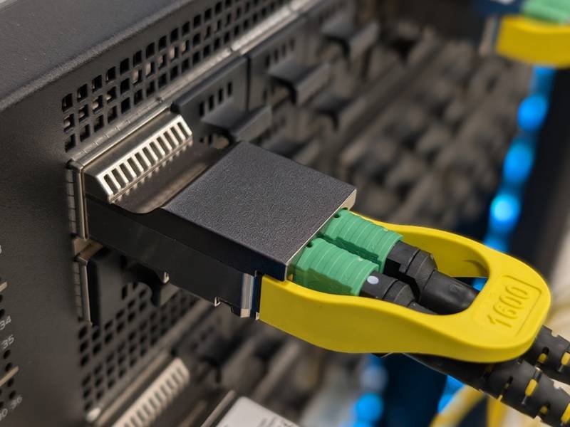
The move from 800G to 1.6T Ethernet looks straightforward on a network diagram: double the port bandwidth, connect the next generation of switches, and keep scaling. At the physical layer, the change is much less tidy. A 1.6T link brings 224G-class electrical signaling, tighter channel-loss budgets, denser front panels, more heat, more demanding connector transitions, and a sharper trade-off between passive copper, active copper, and optics. For AI data centers, the cable is no longer an accessory selected after the switch architecture is finished. It is increasingly part of the electrical, thermal, mechanical, and serviceability design of the system.
The key 1.6T Ethernet interconnect trend is the shift toward eight 200 Gb/s electrical lanes using 224G-class PAM4, combined with shorter passive copper reaches, more active copper options, higher-capacity OSFP and QSFP-DD form factors, and greater use of optical links as distance and thermal demands rise. Interconnect selection is becoming a system architecture decision rather than a simple cable choice.
That shift changes the questions engineers and sourcing teams need to ask. Instead of starting with “Which 1.6T cable should we buy?”, it is more useful to ask where the high-speed electrical path should begin and end, how much loss the host boards consume, what the rack can cool, how the cable will bend behind a dense switch, and what evidence proves that the complete link has enough margin. A cable that performs beautifully on a bench can still be the wrong answer inside a crowded AI rack. The rest of this article follows that real-world decision path, from lane architecture and signal integrity to interconnect selection, form factors, thermal limits, validation, and production control.

What Is Driving 1.6T Ethernet?
1.6T Ethernet is being driven by AI clusters, hyperscale switching, and the need to move more data through each front-panel port without simply doubling the number of cages and cables. The architectural shift toward approximately 200 Gb/s per electrical lane increases bandwidth density, but it also makes signal integrity, power, cooling, routing space, interoperability, and cable architecture much more important than they were at lower lane rates.
AI Fabric Bandwidth
Large AI training and inference systems generate heavy east-west traffic because accelerators repeatedly exchange model parameters, gradients, intermediate results, and memory-related data with other accelerators. When thousands of endpoints participate in a fabric, network congestion can leave expensive compute resources waiting for data. That is why the interconnect is increasingly treated as part of the compute system rather than as a background utility. Moving from 800G to 1.6T gives architects a way to increase bandwidth per port instead of solving every scaling problem by adding more physical ports, cables, and switch layers.
The arithmetic shows the attraction. A nominal 32-port switch at 800G represents 25.6 Tb/s of front-panel bandwidth, while the same nominal port count at 1.6T represents 51.2 Tb/s. Those figures are not application-throughput guarantees, but they explain the pressure toward faster ports. More bandwidth per cage can reduce the number of physical connections required for a given fabric capacity, improve switch radix, and make better use of limited faceplate area. At the same time, the electrical and thermal cost of each port rises, so data-center design becomes a bandwidth-density problem rather than a simple speed race.
Lane Scaling and P802.3dj
The most useful way to understand 1.6T is to separate aggregate Ethernet throughput from the electrical lane architecture. Current 1.6T development is centered on eight electrical lanes carrying roughly 200 Gb/s of Ethernet data per lane with 224G-class PAM4 signaling. That is a major change from the 100G-per-lane electrical generation widely associated with 800G systems. The cable, connector, host board, and SerDes therefore operate with a much tighter high-frequency budget even when the physical port count remains unchanged.
IEEE P802.3dj is the main standards project developing 200 Gb/s-per-lane Ethernet technologies across 200G, 400G, 800G, and 1.6T interfaces. Its scope includes electrical attachment interfaces, backplane links, twinaxial copper cable PMDs, and multiple optical reaches. For 1.6T, important development paths include 1.6TAUI-8, 1.6TBASE-KR8, 1.6TBASE-CR8, and DR-class optical variants. Because the project is still progressing in 2026, engineering documents should identify the specific draft, MSA, host requirement, or supplier qualification baseline rather than treating every product labeled “1.6T” as technically identical.
| Ethernet generation | Representative lane architecture | Approx. data per lane | Aggregate bandwidth |
| 400G | 8 x 50G | 50 Gb/s | 400 Gb/s |
| 800G | 8 x 100G | 100 Gb/s | 800 Gb/s |
| 800G, 224G-class | 4 x 200G | 200 Gb/s | 800 Gb/s |
| 1.6T, 224G-class | 8 x 200G | 200 Gb/s | 1,600 Gb/s |
Bandwidth Density in the Rack
Higher port bandwidth helps AI fabrics scale, but it does not remove physical constraints. A switch with several dozen high-speed ports may have a dense wall of connectors and cables immediately behind the chassis. Larger low-loss copper conductors can improve attenuation, yet they also increase cable diameter and stiffness. Active copper can extend reach, but the electronics in the cable ends add heat. Optical modules reduce the long electrical path, but they move conversion power and thermal load into the front panel. These are system trade-offs, not independent product specifications.
For data-center equipment, the routing path should be considered while the enclosure is still being designed. Available bend space, cable-manager depth, airflow direction, port-row spacing, service loops, and access for replacement all matter. SINO-CONN’s data-center engineering model treats high-density ports, airflow, signal integrity, length management, maintainability, and thermal environment as connected constraints, with twinax, fiber, and high-speed Ethernet considered according to the actual application. That is the right mindset for 1.6T: a link is successful only when it works electrically and still fits, cools, routes, and services correctly in the rack.

How Does 224G PAM4 Change Cable Design?
224G-class PAM4 makes the complete channel less forgiving. Cable attenuation, connector reflections, PCB loss, crosstalk, skew, termination geometry, and manufacturing variation consume a larger share of the available margin. A 1.6T cable therefore cannot be judged by continuity or connector compatibility alone; the cable, connector, PCB launch, SerDes, equalization, and validation method have to be treated as one high-speed transmission system.
Channel Loss and Margin
A high-speed electrical link behaves like a budget in which every part of the path consumes signal quality. The real channel can include the ASIC package, host PCB routing, vias, cage connector, cable termination, twinax section, opposite connector, receiving PCB, and receiver package. At 224G-class signaling, the frequency-dependent losses and discontinuities in those elements become more difficult to tolerate. IEEE 802.3dj work has used a die-to-die insertion-loss baseline around 40 dB at approximately 53.125 GHz for the relevant 200G-per-lane CR/KR families, which illustrates how tightly the complete channel must be managed.
That figure should not be misread as a cable-only allowance. If the two host boards consume too much of the available budget, a low-loss DAC may still have little usable reach. Conversely, improving the ASIC-to-cage route can create more room for cable length without changing the external cable. This is one reason near-ASIC cabling and lower-loss board architectures are gaining attention. Engineers should allocate loss across package, PCB, connector, cable, temperature, and manufacturing tolerance before the mechanical design is frozen. Quoting only the cable insertion loss gives an incomplete picture of whether the final system will be robust.
SI Metrics That Matter
No single signal-integrity metric is enough to qualify a 1.6T electrical channel. Insertion loss describes attenuation, while return loss exposes reflections caused by impedance discontinuities. Differential impedance helps show whether the transmission geometry is controlled, but a good nominal impedance does not guarantee low loss or low crosstalk. Crosstalk becomes more important when many high-speed lanes are packed into one connector and cable end, and skew can convert part of a differential signal into common-mode energy if the two conductors do not remain electrically matched.
BER provides the system-level consequence of all those effects, but it should be interpreted alongside passive measurements and FEC behavior. SINO-CONN’s high-speed engineering framework connects protocol, data rate, channel count, pair geometry, shielding, return path, skew, insertion loss, return loss, and BER to one validation plan instead of treating them as separate checkboxes. That approach is especially important at 224G-class rates, where a cable may pass continuity, look mechanically correct, and still fail because the high-frequency channel has too little margin.
Connector and Termination Control
The middle of a controlled twinax cable is often more predictable than the few millimeters around the connector. In the termination zone, conductors leave the cable structure, shielding may open, pair spacing changes, contacts introduce new geometry, and the return path transitions into the connector and PCB. Excess exposed conductor length, inconsistent shield cutback, long solder tails, asymmetric routing, or poor ground placement can create reflections and mode conversion even when the bulk cable itself is excellent.
This is where manufacturing discipline becomes part of signal integrity. A prototype assembled by an experienced technician may perform well because the conductor placement is carefully adjusted by hand. That result is not scalable unless the critical geometry is converted into drawing dimensions, fixtures, work instructions, controlled stripping lengths, shield-termination rules, and inspection points. For impedance-controlled high-speed assemblies, SINO-CONN’s internal engineering process specifically treats connector transitions, PCB transitions, stripping length, shield termination, and overmold regions as potential discontinuities that require controlled structure and project-specific validation when the application demands it.
FEC and Equalization
FEC, transmitter equalization, receiver equalization, and link training are fundamental to modern high-speed Ethernet, but they should not be treated as permission to accept a poor physical channel. Equalization can compensate for predictable loss, and FEC can correct a defined level of errors, yet neither provides unlimited recovery. A safer engineering sequence is to remove avoidable physical loss first, control reflections and crosstalk, preserve differential symmetry, keep enough receiver margin, and then use equalization and FEC within their intended operating range.
A link that comes up once is not necessarily a healthy link. A marginal cable may work on one switch at room temperature and fail after the port warms up, after another cable lot is installed, or when it is connected to a host with slightly different SerDes behavior. Pre-FEC error behavior is therefore valuable because it shows how hard the correction system is working before errors are hidden. Some current 1.6T AEC products publish both pre-FEC and post-FEC BER values, which is a useful example of how serious high-speed qualification distinguishes raw channel behavior from corrected system behavior.

Which Interconnects Fit 1.6T?
No single interconnect is best for every 1.6T link. Passive DAC is attractive for very short connections because it adds almost no cable-side power or latency. ACC and AEC extend electrical reach by adding signal conditioning or retiming. AOC and pluggable optics become more attractive as distance, routing, and cable bulk increase. The correct choice comes from the full reach, loss, thermal, serviceability, and cost budget.
Passive DAC
Passive direct-attach copper remains difficult to beat when the required connection is short and both hosts are designed for the electrical channel. Because the cable contains no active retimer or optical conversion, it can offer extremely low cable-side power consumption, very low added latency, simple replacement, and potentially lower component cost. The continued development of 1.6TBASE-CR8 confirms that passive twinax remains part of the 1.6T Ethernet roadmap rather than disappearing simply because lane rates have doubled.
The limiting factor is electrical reach. At 200 Gb/s per lane, cable length cannot be discussed independently from conductor gauge, host PCB loss, connector design, and the available channel budget. Thicker conductors may reduce attenuation, but they increase outside diameter, stiffness, and bend radius. Shorter cable improves margin, but it can restrict rack layout. For passive 1.6T projects, the useful question is not “What is the maximum DAC length?” in isolation. The better question is “How much insertion-loss budget remains for the cable after both host channels, connectors, and operating conditions are included?”
ACC and AEC
Active copper is useful when designers want to keep the operational simplicity of a copper assembly but passive loss has become too difficult. ACC generally uses analog conditioning or equalization, while AEC commonly uses retimers that recover and retransmit the signal. A retimed AEC can effectively break one difficult electrical path into shorter controlled segments, creating more reach or host margin than a passive cable. This can be valuable in top-of-rack, accelerator, and high-density switch environments where a few meters of copper are still operationally attractive.
The trade-off is that the cable becomes an active electronic device. Power consumption, heat, firmware, management, interoperability, and latency all become part of the selection process. Current commercial 1.6T AEC products demonstrate practical OSFP-to-OSFP implementations in roughly one-to-three-meter classes, but vendor-specific reach should not be treated as a universal industry limit. AEC can be a strong middle option when passive copper is marginal and optics adds unnecessary complexity, yet the decision should be made at the system level rather than from a single headline reach number.
AOC and Pluggable Optics
AOC moves the long portion of the connection into the optical domain while keeping a cable-like installation experience. Electrical-to-optical conversion occurs at the cable ends, and the fiber section avoids the increasing attenuation associated with carrying 224G-class electrical signals over a longer copper path. This can reduce cable weight, improve routing flexibility, and extend practical reach. The main operational trade-off is that the optical engines and fiber are usually replaced as one integrated assembly rather than as separate service components.
Pluggable optical modules separate the transceiver from the fiber plant, which is often preferable when operators need multiple reaches, structured fiber cabling, independent module replacement, or longer rack-to-rack and data-hall connections. Current 1.6T Ethernet development includes both copper and DR-class optical paths, which is a useful reminder that the market is not choosing one universal medium. The electrical-to-optical boundary is being placed according to reach, thermal design, service strategy, cost, and the amount of electrical channel margin available before conversion.
System-Level Selection
The best interconnect is the one that solves the full deployment problem with enough margin, not the one that wins a single metric. Passive DAC may have the lowest cable power, but only if the distance and host design make it viable. AEC may extend copper reach, but its active ends can add substantial heat. AOC and optics can simplify long-distance signal transport, but they add conversion electronics and different service requirements. Total cost also includes cooling, installation, replacement time, port failures, and the operational burden of troubleshooting marginal links.
| Interconnect | Typical 1.6T role | Active electronics | Main advantage | Main constraint |
| Passive DAC | Very short electrical links | No | Lowest cable-side power and minimal added latency | Tight 224G channel-loss budget |
| ACC | Short active copper links | Analog conditioning | Extends electrical usability with less complexity than full retiming | Product-specific reach and interoperability |
| AEC | Short-to-medium active copper links | Retimer | Restores signal and relaxes passive channel limits | Power, heat, firmware, and latency |
| AOC | Medium optical cable-style links | Optical conversion | Lower cable bulk and longer practical reach | Whole assembly is usually replaced together |
| Pluggable optics | Rack-to-rack and longer links | Optical transceiver | Broad reach and service flexibility | Module power, cost, and front-panel thermals |
A practical sourcing comparison should therefore include watts per port, expected reach, cable diameter, bend behavior, field replacement method, host compatibility, validation evidence, and the total link cost per delivered bandwidth. A cable with a higher purchase price can be cheaper at the system level if it reduces cooling, avoids signal-debug work, simplifies routing, or prevents unstable ports. Conversely, using optics on a very short link can add power and cost without delivering meaningful system value. The architecture should follow the actual constraints.
How Are 1.6T Form Factors Evolving?
1.6T form factors are evolving around eight high-speed electrical lanes, higher thermal capacity, tighter signal-integrity control, and flexible breakout. OSFP and QSFP-DD1600 are both important platforms, while near-ASIC cabling and co-packaged approaches are shortening the difficult electrical path. The broader trend is not simply a new connector shape; it is moving the electrical boundary closer to the switch silicon as lane rates increase.
OSFP at 1.6T
OSFP is an important 1.6T platform because its architecture accommodates eight high-speed differential lanes and provides a mechanical envelope designed for demanding thermal conditions. Current OSFP specifications support 1.6TAUI-8 with eight 224G-class PAM4 electrical lanes carrying approximately 200 Gb/s of Ethernet data per lane. The same eight-lane structure can also support lower aggregate rates through lane grouping when the host ASIC and firmware allow the required mapping, which makes the form factor useful during mixed-generation deployments.
This flexibility can support configurations such as one 1.6T port, two 800G links, four 400G links, or eight 200G-class paths. That does not mean every OSFP port automatically supports every breakout mode. Lane mapping, ASIC capability, FEC configuration, module management, firmware, and the cable or module architecture must agree. Mechanical compatibility is only the first layer. For 1.6T, the host PCB, connector transition, termination, module power, and thermal environment remain part of the same qualification problem.
QSFP-DD1600
QSFP-DD also continues into the 1.6T generation. QSFP-DD1600 is an eight-lane architecture designed around approximately 200 Gb/s electrical lanes for 1.6 Tb/s aggregate bandwidth, with updated signal-integrity and thermal provisions for the higher-speed environment. That matters because 1.6T is not developing around a single mechanical winner. Different switch platforms can make different trade-offs between front-panel density, cooling headroom, host routing, existing platform compatibility, cage design, service strategy, and supplier ecosystem.
For cable development, the form factor should be frozen early because the connector, high-speed termination, shell, ground structure, and mechanical exit geometry can affect electrical behavior. Choosing the form factor late and treating it as an interchangeable end fitting is risky at 224G-class signaling. A supplier may be able to build both OSFP and QSFP-DD families, but each construction still needs its own controlled drawing, termination method, validation limits, and manufacturing baseline. Port density alone should never be used as proof that the electrical channel has enough margin.
Breakout Architecture
Breakout becomes especially valuable when switch and endpoint generations do not migrate at the same time. A new 1.6T switch may need to connect to 800G, 400G, or 200G devices for several product cycles. Because the 1.6T host architecture contains multiple high-speed lanes, those lanes can be grouped into lower-rate logical ports when the ASIC and interface specifications support it. This can make a single 1.6T cage much more useful during staged infrastructure upgrades.
A breakout assembly is not simply one large connector splitting into several smaller ones. Each branch has to preserve correct transmit and receive mapping, high-speed lane identity, ground reference, pair geometry, shield continuity, branch length, connector orientation, and mechanical strain relief. In production, branch identification and revision control become critical because several branches may look nearly identical. For large deployments, stable part numbers, serialized or batch-controlled labels, and a clear electrical lane map can save substantial commissioning time and reduce the chance that a mechanically correct cable is connected to the wrong logical port.
Near-ASIC and Co-Packaged Links
The most important form-factor trend may be happening behind the front panel. At 224G-class signaling, long PCB routes between the switch ASIC and the cage consume a valuable portion of the electrical budget before the external interconnect even begins. Near-ASIC cable systems shorten that board path by moving a controlled cable interface closer to the silicon. Co-packaged copper takes the same principle further, while co-packaged optics moves optical conversion close to the ASIC so that the longest path no longer carries the highest-speed electrical signal.
These architectures can reduce electrical loss and potentially lower dependence on expensive ultra-low-loss PCB materials, but they introduce new challenges in assembly, cooling, serviceability, test access, and repair. A pluggable module at the front panel is easy to replace; a deeply integrated optical or electrical interface may not be. The trend should therefore be understood as a shift in where the electrical boundary is placed, not as proof that pluggable optics will disappear. As lane rates continue to increase, shortening the electrical path will remain one of the most effective ways to preserve system margin.
What Limits 1.6T Deployment?
1.6T deployment is limited mainly by electrical loss, thermal density, cable routing, and interoperability rather than by nominal bandwidth alone. Passive copper loses reach as 224G-class channels consume more loss budget, while active copper and optics add port power. Larger low-loss copper cables can also restrict airflow and bending space. A reliable link therefore has to work electrically, mechanically, thermally, and across the real host ecosystem.
Copper Reach and Loss
Copper reach becomes more difficult as signaling frequency rises because conductor loss, dielectric loss, connector discontinuity, crosstalk, and mode conversion all become more significant. A longer cable is not the only source of loss. The package, host board, vias, cage, cable plug, opposite host path, and temperature all contribute to the end-to-end result. That is why maximum cable length cannot be treated as a universal number that applies to every 1.6T host pair.
Wire gauge illustrates the trade-off clearly. Larger conductors can reduce attenuation, but they increase cable diameter and stiffness. That may improve electrical reach while making the rack harder to cable, reducing bend flexibility, and obstructing cooling air. The better engineering target is the lowest practical total channel loss, not simply the lowest cable loss. In many cases, shortening the host PCB route, improving connector transitions, or moving the electrical boundary closer to the ASIC can create more useful margin than making the external copper cable dramatically thicker.
Power and Thermal Density
Active interconnects solve signal problems by adding electronics, and electronics turn part of the problem into heat. This is particularly important at the front panel, where high-speed ports are densely packed and cooling air is already constrained by cages, heat sinks, connectors, and cable bundles. One current commercial 1.6T retimed AEC product brief lists roughly 24 W per cable end. That is a product-specific figure rather than a generic requirement, but it shows why active cable power cannot be ignored in a dense 1.6T design.
If thirty-two active cable ends consumed 24 W each, the arithmetic would be 768 W of cable-end electronics. A real system may use a very different power figure or topology, yet the example shows how quickly the thermal burden can become material. Engineers should compare watts per port, watts per delivered terabit, inlet temperature, module case temperature, fan power, adjacent-port heating, and cable obstruction. A solution that provides excellent electrical margin but requires significantly more cooling may not deliver the best system efficiency.
Cable Bulk and Airflow
Mechanical dimensions should be reviewed before rack layout is frozen because cable diameter and bend radius scale into real space surprisingly quickly. One published 1.6T AEC family provides a useful product-specific reference: examples list cable outside diameters around 8.2 mm for 32 AWG, 9.0 mm for 30 AWG, and 9.9 mm for 28 AWG, with minimum static bend radii in the roughly 43-49 mm range. These values are not universal, but they illustrate the physical price of using heavier copper construction.
| Example gauge | Example cable OD | Example minimum static bend radius | Practical rack implication |
| 32 AWG | 8.2 mm | 43 mm | Smaller bundle, easier routing, but higher electrical loss than heavier gauges |
| 30 AWG | 9.0 mm | 43 mm | Middle ground between loss and cable bulk |
| 28 AWG | 9.9 mm | 49 mm | Lower-loss potential, but more bundle volume and bend clearance |
The difference between an 8.2 mm and 9.9 mm cable may look minor when one cable is held in the hand. Across dozens of ports, the bundle cross-section, stiffness, and required turning space become much more significant. Rear-door clearance, horizontal cable managers, vertical trays, fan exhaust, and service loops all need enough space. SINO-CONN’s engineering framework treats bend radius and routing as design inputs because excessive bending can damage shielding, change high-speed geometry, load connector exits, or create intermittent reliability problems even when the initial electrical test passes.
Interoperability and Margin
Interoperability matters more as margin shrinks because two products can support the same nominal data rate and still behave differently when connected. Host SerDes tuning, transmitter equalization, receiver equalization, FEC settings, cable response, CMIS behavior, firmware, link training, and temperature can all affect the result. A cable that works on one switch-NIC pair may not provide the same margin on another combination, especially if the first system has unusually strong equalization or a shorter internal board route.
A stronger qualification process asks which host platforms were tested, what cable lengths were used, whether pre-FEC behavior was measured, what temperatures were covered, whether multiple production samples were compared, and which firmware or module-management versions were involved. Multi-vendor interoperability events are valuable because they expose differences that a single-vendor bench test can hide. For a large deployment, “the link came up” is only the beginning. Stable operation under sustained traffic, realistic temperature, production variation, and multiple hosts provides a much more useful picture of actual deployment margin.
How Should Engineers Prepare for 1.6T?
Engineers should prepare for 1.6T by defining the complete channel before choosing the cable. Start with data rate, lane mapping, host interface, connector, length, routing, thermal environment, and acceptance criteria. Prototype the actual construction, characterize passive signal integrity and system behavior, then freeze drawings, BOMs, termination geometry, test methods, and revision controls before scaling into production. That process is more reliable than selecting by bandwidth label alone.
Define the Channel First
A request that says only “1.6T cable, two meters” does not contain enough information for serious engineering. The interconnect supplier needs to understand the host architecture and the environment in which the cable will operate. Useful inputs include the target Ethernet mode, lane configuration, exact form factor, host platform, cable length, passive or active preference, breakout mapping, available bend space, operating temperature, port density, airflow direction, applicable IEEE or MSA baseline, and the SI or BER criteria that will be used to release the design.
Mechanical information can be as valuable as electrical information. A chassis drawing, STEP file, rear-rack photograph, or dimensioned routing sketch may show that a proposed cable cannot bend behind the switch long before samples are manufactured. SINO-CONN’s engineering process treats protocol, data rate, channel count, connector, allowed length, pair geometry, shielding, return path, routing, and validation requirements as connected inputs. For emerging 1.6T constructions, that kind of front-loaded definition reduces sample loops and helps prevent a technically fast cable from becoming a mechanically unusable one.
Useful project inputs normally include:
- Target Ethernet rate and lane configuration.
- Host connector or form factor and exact part number where available.
- Switch, NIC, accelerator, or test platform information.
- Required cable length and breakout mapping.
- Available bend space, exit direction, and routing path.
- Operating and storage temperature range.
- Port density and airflow direction.
- Shielding and grounding requirements.
- Applicable IEEE draft, MSA, or customer specification.
- Required SI, BER, traffic, and reliability tests.
- Prototype quantity, pilot plan, and expected production volume.
Build the Validation Plan
The validation plan should be written before the prototype arrives. Otherwise, teams often receive a sample and only then begin deciding what “pass” means. A practical sequence starts with manufacturing correctness: connector identity, lane mapping, polarity, opens and shorts, overall dimensions, breakout dimensions, and shield or ground termination. The next layer is passive high-speed behavior, which may include impedance profile, insertion loss, return loss, crosstalk, skew, and verification of the test fixture and reference planes.
The final layer is operation on the real system. That can include link establishment, negotiated mode, sustained traffic, pre-FEC error behavior, post-FEC counters, elevated-temperature operation, and multi-host compatibility where required. Not every project needs every test, and a good plan avoids testing for the sake of generating reports. The method should match the expected failure mechanisms. A continuity tester proves wiring correctness but not 1.6T performance. A VNA characterizes the passive channel but does not prove every host will operate. System traffic proves operation on the tested platform but may not reveal how much signal-integrity margin remains.
Prototype to Production
A successful engineering sample is not yet a production-ready high-speed cable. A skilled technician can manually control shield cutback, pair position, solder geometry, and cable exit angle while making a handful of prototypes. Those details become dangerous when they remain in the technician’s hands instead of being transferred into controlled documentation. At 224G-class signaling, a few millimeters of extra exposed conductor or an altered ground transition can have more impact than a much larger cosmetic change elsewhere in the assembly.
Production readiness therefore requires a released drawing, controlled BOM, approved connector and cable part numbers, termination dimensions, shield-cutback limits, work instructions, fixtures, inspection criteria, golden or approved samples, and a defined change-control process. SINO-CONN’s engineering workflow connects drawing development, BOM control, DFM, DFT, prototype validation, pilot production, and repeat manufacturing so that the successful sample becomes a repeatable process rather than a one-time craft result. For 1.6T projects, repeatability is a performance requirement because manufacturing variation can consume the same signal margin that the electrical design worked hard to preserve.
Supplier Evidence and Future Scaling
A credible high-speed supplier should be evaluated by the engineering evidence it can produce, not by the number of protocol names on its website. Useful evidence includes controlled drawings, lane maps, connector and cable identification, BOM revisions, shield and ground definitions, critical termination dimensions, test requirements, fixture information, validation reports, prototype revision history, production inspection plans, lot identification, and change-control records. The strongest statement is not “we make high-speed cables”; it is that a specific construction has been built and validated against a defined host, channel, and acceptance plan.
That discipline is also the best preparation for the generation after 1.6T. Industry work is already exploring 400G-per-lane electrical technologies, which will place even more pressure on electrical path length, connector transitions, cooling, packaging density, and measured validation. Today’s 1.6T work is therefore a useful transition point. Teams that learn to define, measure, document, and control the complete channel will be better prepared for future speeds than teams that rely on a simple bandwidth label. The engineering process becomes the reusable asset, even as the exact connector, lane rate, and medium continue to change.
Conclusion
1.6T Ethernet is not simply an 800G cable with twice the number printed on the label. It changes the relationship between SerDes, host PCB, connector, cable construction, active electronics, optics, thermal design, rack routing, and production control. Passive DAC will remain valuable where the electrical path is short enough. Active copper will fill links where passive margin is insufficient but copper still makes operational sense. AOC and pluggable optics will become increasingly important as distance, cable bulk, and electrical loss grow, while near-ASIC and co-packaged architectures will continue pushing the high-speed boundary closer to the silicon. For engineering teams, the durable strategy is straightforward: define the complete channel, quantify the real constraints, validate the chosen architecture, and then lock the manufacturing process so the production cable behaves like the approved prototype.
Frequently Asked Questions
Is 1.6T Ethernet the same as 1.6 TB/s?
No. 1.6T Ethernet normally refers to an aggregate line rate of about 1.6 terabits per second, written as 1.6 Tb/s. A byte contains eight bits, so 1.6 Tb/s corresponds to a theoretical raw rate of about 200 gigabytes per second before protocol overhead and other system effects are considered. In practice, application throughput is lower because Ethernet framing, FEC, protocol overhead, host architecture, and traffic behavior all affect the usable payload rate. Mixing Tb/s and TB/s can therefore create an eightfold misunderstanding in bandwidth calculations.
Does 1.6T Ethernet require 224G PAM4 lanes?
Current mainstream 1.6T development is based on 224G-class PAM4 electrical signaling with approximately 200 Gb/s of Ethernet data per lane and eight lanes for a 1.6 Tb/s aggregate interface. The term “224G” describes the electrical signaling generation rather than a simple 224 Gb/s payload number. Engineers should still verify the exact interface specification because host attachment, PMD type, FEC, lane mapping, and the applicable IEEE or MSA revision determine the final implementation. A product labeled 1.6T should not be assumed to use the same electrical architecture as every other 1.6T product.
How far can a passive 1.6T DAC reach?
There is no universal passive 1.6T DAC length that applies to every host pair. Practical reach depends on the complete channel budget, including package loss, host PCB routing, vias, cage and connector transitions, cable gauge, termination construction, temperature, and receiver equalization. IEEE 1.6TBASE-CR8 work confirms that passive twinax is part of the 1.6T roadmap, but a usable cable length still has to be evaluated against the specific host architecture and cable construction. For this reason, a credible supplier should ask for host and channel information rather than promise one maximum length for every application.
What is the difference between DAC, ACC, and AEC at 1.6T?
A passive DAC contains no active signal-processing electronics and is generally preferred when the electrical path is short enough because it offers very low power and latency. ACC adds analog conditioning or equalization to improve the electrical signal without the same full retiming behavior as a typical AEC. AEC commonly uses retimers to recover and retransmit the signal, which can extend practical copper reach but adds power, heat, firmware, interoperability considerations, and some latency. The correct choice depends on the host loss budget, distance, thermal limits, and operating priorities rather than on the product name alone.
Is OSFP the only form factor for 1.6T Ethernet?
No. OSFP is an important 1.6T platform because it supports eight high-speed electrical lanes and provides useful thermal capacity, but QSFP-DD1600 is also part of the 1.6T ecosystem. Different equipment vendors can choose different form factors according to front-panel density, cooling, host PCB routing, backward compatibility, cage design, and their existing module strategy. Engineers should therefore specify the actual form factor and host platform during cable development. Mechanical compatibility by itself does not prove electrical compatibility at 224G-class lane rates.
What tests are most useful for a 1.6T cable assembly?
The most useful tests depend on the architecture, but a serious program usually separates manufacturing correctness from high-speed performance. Manufacturing checks include lane mapping, continuity, opens and shorts, dimensions, and shield or ground termination. High-speed characterization may include TDR or impedance profile, insertion loss, return loss, crosstalk, and skew. System validation can add link establishment, sustained traffic, pre-FEC and post-FEC error behavior, temperature testing, and multi-host interoperability. No single test proves everything, so the acceptance plan should combine the measurements that correspond to the actual failure risks.