Skip to content
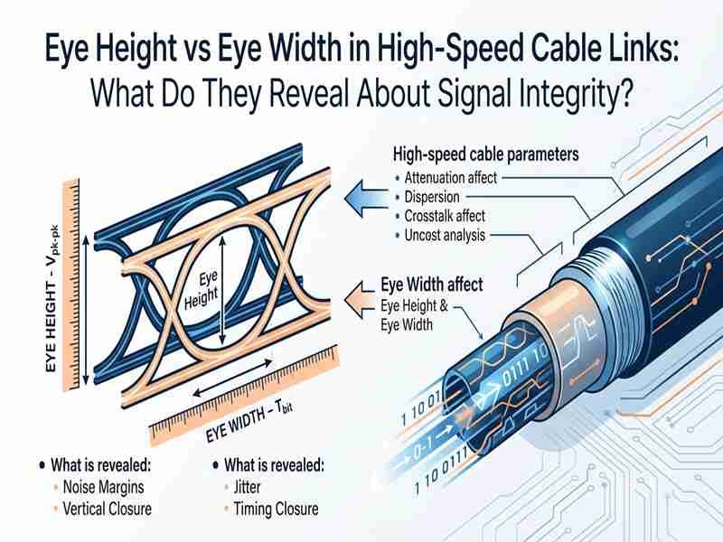
A high-speed cable can pass continuity testing, show the correct pinout, and look perfectly assembled, yet still fail as soon as the data rate or cable length increases. That is where an eye diagram becomes much more useful than a basic pass-or-fail electrical check. The eye does not merely show whether a waveform looks clean. Its vertical and horizontal openings reveal two different kinds of operating margin, and the difference between them can point engineers toward very different root causes.
Eye height is the vertical opening of an eye diagram and mainly reflects usable voltage or amplitude margin, while eye width is the horizontal opening and mainly reflects timing margin. In a high-speed cable link, reduced eye height often points toward loss or noise, while reduced eye width often points toward jitter or timing uncertainty. Both can shrink together because ISI, reflections, crosstalk, and channel loss affect amplitude and edge timing at the same time.
The practical value comes from reading both dimensions together instead of treating an eye screenshot as a beauty contest. Imagine two cable prototypes on the same test platform: one keeps generous vertical opening but has a narrow sampling window, while the other preserves timing but loses amplitude. Calling one simply better misses the engineering story. Their eyes are telling you that the links are running out of margin in different ways, and that distinction can save hours of trial-and-error debugging before the design reaches production.

What Are Eye Height and Eye Width?
Eye height is the vertical opening of an eye diagram and mainly reflects available voltage or amplitude margin. Eye width is the horizontal opening and mainly reflects timing margin. Both matter in a high-speed cable link because loss, noise, jitter, reflections, crosstalk, and inter-symbol interference can reduce the receiver’s ability to distinguish both the correct signal level and the safe sampling time.
Eye Height and Voltage Margin
Eye height describes how much vertical separation remains between the upper and lower signal distributions around the receiver’s sampling region. It is normally expressed in volts or millivolts, although the exact definition depends on the oscilloscope, compliance procedure, statistical contour, and measurement settings. In practical terms, a larger vertical opening usually gives the receiver more room to distinguish one amplitude state from another before noise, loss, ringing, or other disturbances push the signal toward the decision threshold.
Eye height should not be confused with peak-to-peak signal amplitude. Two links can have similar nominal swing while producing very different usable vertical openings because one contains more noise, overshoot, crosstalk, or pattern-dependent variation. If one cable produces 300 mV of eye height and another produces 150 mV under the same transmitter, receiver, fixture, pattern, equalization, and measurement method, the first link has more vertical margin. The comparison becomes unreliable once those conditions change, so eye height is best treated as a controlled margin measurement rather than a universal pass number.
Eye Width and Timing Margin
Eye width describes the horizontal time window in which the receiver can sample a symbol with acceptable confidence. It is commonly expressed in picoseconds or as a fraction of one unit interval, or UI. One UI is simply one symbol period, so the available time becomes dramatically smaller as symbol rate increases. At 10 GBd, one UI is 100 ps; at 25 GBd, it is 40 ps; at 56 GBd, it is only about 17.86 ps. A timing disturbance that once looked insignificant can therefore consume a large share of the decision window in a faster link.
This makes eye width especially useful when engineers are dealing with jitter, skew, data-dependent edge movement, duty-cycle distortion, clock recovery, and ISI. At 25 GBd, an eye width of 0.60 UI corresponds to about 24 ps. If another 0.10 UI disappears because of jitter or reflections, roughly 4 ps of timing margin is gone. The number is small in everyday terms, but it is large relative to a high-speed receiver’s sampling window. Eye width is therefore not just a visual measure of a wide or narrow eye; it is a direct way to think about how much timing uncertainty the link can still tolerate.
| Symbol Rate | 1 UI | 0.50 UI | 0.25 UI |
| 5 GBd | 200 ps | 100 ps | 50 ps |
| 10 GBd | 100 ps | 50 ps | 25 ps |
| 25 GBd | 40 ps | 20 ps | 10 ps |
| 32 GBd | 31.25 ps | 15.63 ps | 7.81 ps |
| 56 GBd | 17.86 ps | 8.93 ps | 4.46 ps |

Voltage Margin vs Timing Margin
A useful first interpretation is simple: eye height is mainly about voltage margin, while eye width is mainly about timing margin. That distinction helps engineers organize the problem, but it should not be treated as a rigid law. A reflection, for example, can alter amplitude at one point in the pattern and also shift the time at which an edge crosses the receiver threshold. ISI can lower the voltage reached by one symbol and move the timing of the next transition, so the same physical defect can reduce both dimensions.
This is why experienced signal-integrity teams rarely diagnose a cable link from one eye number. Eye height and eye width become much more useful when they are correlated with insertion loss, return loss, TDR, crosstalk, skew, equalization settings, and BER. The eye tells you what kind of margin is disappearing at the receiver; the supporting measurements help explain what in the channel is consuming that margin. When those views agree, troubleshooting becomes far more focused than simply replacing the cable and hoping the next sample looks better.
Is a Bigger Eye Always Better?
Under identical conditions, more eye opening normally means more margin, but a visually larger eye does not automatically prove that a cable assembly passes the required interface. A raw waveform captured before receiver equalization can look heavily closed while the actual receiver still recovers the data successfully. The opposite can also happen: a generous-looking eye produced with favorable transmitter settings, a short repetitive pattern, or aggressive display scaling may hide the conditions that dominate real operation.
Meaningful comparison requires the same data rate, cable length, connector configuration, transmitter amplitude, equalization, pattern, fixture, measurement point, bandwidth, de-embedding method, and BER criterion. If those conditions differ, the screenshots may still be interesting, but they are not clean evidence that one cable is better. The practical question is not which cable produces the prettiest eye. It is which cable retains enough vertical and horizontal margin under the conditions that represent the real transmitter-channel-receiver system, including the manufacturing and environmental variation that the product must tolerate.
Which Effects Reduce Eye Height or Eye Width?
Eye height is commonly reduced by attenuation, noise, crosstalk, and amplitude distortion, while eye width is commonly reduced by jitter, skew, and timing displacement. Real cable impairments often affect both dimensions at once. Frequency-dependent loss creates ISI, reflections change amplitude and edge timing, and crosstalk can appear as both vertical noise and deterministic jitter, so diagnosis should consider the complete channel rather than one metric alone.
Noise, Loss, and Vertical Closure
A passive copper cable does not transmit every frequency component equally. Conductor loss, dielectric loss, skin effect, and other channel mechanisms generally make insertion loss rise with frequency. Since fast digital edges depend on higher-frequency content, the received waveform becomes smaller, slower, and more distorted as the channel gets longer or lossier. The first visible symptom may be reduced amplitude, which directly consumes eye height, but the deeper problem is that a bandwidth-limited waveform also takes longer to settle between symbols.
Noise consumes whatever vertical margin remains. Sources can include adjacent high-speed pairs, switching power circuits, external EMI, receiver noise, imperfect shielding, and disturbances on the return path. The practical concern is not simply how much nominal signal swing remains, but how far the statistical signal distributions stay from the receiver threshold under realistic conditions. A link with 180 mV of apparent vertical opening and 20 mV of disturbance has a very different risk profile from one with similar nominal opening but 70 mV of disturbance. Once loss slows the edges enough to create ISI, the original vertical problem begins to reduce eye width as well.
Jitter, Skew, and Horizontal Closure
Jitter is variation in transition timing. Instead of every edge arriving at exactly the ideal instant, real edges arrive slightly early or late. Random jitter is associated with stochastic processes such as thermal and phase noise, while deterministic jitter can come from periodic interference, duty-cycle distortion, reflections, crosstalk, and pattern-dependent channel behavior. As the distribution of crossing times spreads, the horizontal sampling window becomes narrower even when the vertical signal levels remain relatively strong.
Skew creates a related problem. In a differential pair, the positive and negative conductors should remain closely matched in electrical length. Unequal conductor lengths, asymmetrical dielectric exposure, termination geometry, or connector routing can create intra-pair skew, while multi-lane links may also be sensitive to pair-to-pair skew. The same absolute error becomes more serious as symbol rate rises: a 5 ps timing shift uses 5% of one UI at 10 GBd, 12.5% at 25 GBd, 16% at 32 GBd, and about 28% at 56 GBd. That is why tiny geometric differences can become real electrical constraints.
ISI and Pattern Dependence
Inter-symbol interference means that the waveform produced by the current symbol depends partly on symbols that came before it. A bandwidth-limited channel cannot settle instantly, so a one following a long run of zeros may reach a different voltage and cross the receiver threshold at a different time than a one embedded in an alternating pattern. The channel effectively has memory, and the eye diagram reveals that memory by overlaying many different symbol histories on top of one another.
ISI reduces eye height because the receiver sees several possible amplitudes for what is nominally the same logical level, and it reduces eye width because threshold crossings move according to the surrounding data pattern. This is why a cable can look acceptable with an easy repetitive sequence yet perform poorly with a more stressful pseudorandom pattern. Equalization techniques such as transmitter FFE, receiver CTLE, and DFE are largely designed to compensate for this predictable channel memory. When the eye improves strongly after equalization, that tells the engineer something important about the role of frequency-dependent loss and ISI in the original closure.
Crosstalk and Reflections
Crosstalk occurs when electromagnetic energy from one signal path couples into another. In a multi-pair cable, dense connector, or compact harness, an aggressor channel can inject unwanted energy into a neighboring victim channel. Depending on geometry, spacing, shielding, frequency, and switching pattern, the disturbance may appear as vertical noise, shifted edge timing, or both. That makes crosstalk a common reason for an eye that looks acceptable when only one lane is active but degrades when neighboring channels begin switching.
Reflections create similarly mixed behavior. When a signal encounters an impedance discontinuity, part of its energy continues forward and part reflects. The delayed reflected energy can combine with the main waveform to create ringing, overshoot, undershoot, amplitude ripple, or pattern-dependent edge displacement. Typical physical sources include excessive pair untwist, long exposed conductors, stubs, connector launches, abrupt cable geometry changes, and inconsistent shield termination. In high-speed cable work, these are not merely workmanship details. The mechanical geometry forms part of the transmission line, which is why a cable that passes continuity can still lose both eye height and eye width at speed.
What Does Uneven Eye Closure Mean?
Uneven eye closure is a useful diagnostic clue. A tall but narrow eye often points toward timing problems such as jitter, skew, or data-dependent edge movement. A short but wide eye more strongly suggests amplitude loss or noise. When both dimensions deteriorate, engineers should investigate broader channel impairments such as insertion loss, ISI, reflections, crosstalk, or insufficient equalization rather than assuming one isolated fault.
Good Height, Poor Width
A cable link with strong vertical opening but limited horizontal opening still gives the receiver enough amplitude to distinguish signal levels, but the safe sampling window is becoming fragile. This pattern often turns attention toward random or deterministic jitter, intra-pair skew, pair-to-pair skew, data-dependent timing variation, clock recovery, asymmetric rise and fall behavior, reflections near sensitive transitions, or insufficient compensation for ISI. The waveform can look tall and healthy to the eye while carrying very little timing headroom.
Suppose a 25 GBd channel retains 320 mV of eye height but only 0.30 UI of eye width. The vertical margin may look comfortable, yet 0.30 UI at 25 GBd is only 12 ps. A few additional picoseconds caused by temperature, connector variation, PCB routing, silicon package effects, or production tolerance can consume a large fraction of what remains. That is why increasing conductor size or transmitter swing may do little for this failure pattern. Before changing the cable construction, it is usually more productive to look at jitter decomposition, skew, threshold-crossing behavior, reflections, and the effect of receiver equalization.
Poor Height, Good Width
A short but relatively wide eye tells a different story. Transition timing remains comparatively stable, but the difference between signal levels is shrinking. Typical investigation areas include excessive insertion loss, insufficient transmitter swing, vertical noise, crosstalk, common-mode disturbance, lossy connector transitions, amplitude-related reflections, and receiver sensitivity. Cable length is a particularly useful diagnostic variable because a strong reduction in eye height with increasing length often points toward a channel-loss problem before it points toward a pure timing problem.
The critical question is how much vertical margin remains under worst-case conditions, not whether one room-temperature prototype still works. A link that passes with only a modest vertical opening may become fragile when conductor loss changes with temperature, connector contact behavior varies, receiver sensitivity shifts across silicon, or production geometry moves within tolerance. Robust engineering therefore looks for margin across realistic variation rather than a single passing screenshot. If the eye stays wide while becoming progressively shorter with cable length, insertion loss, noise, and receiver amplitude requirements deserve early attention.
Both Height and Width Are Poor
When both dimensions collapse, the channel usually has a broader signal-integrity problem or has simply reached the limit of its available channel budget. Frequency-dependent loss is a common example: the signal becomes smaller because of attenuation, while the loss of high-frequency content slows the edges and increases ISI. Severe reflections can produce amplitude ripple and delayed energy, while crosstalk can add noise and move crossing times. These mechanisms naturally affect both axes rather than staying inside a single vertical or horizontal category.
The most useful response is to stop treating the eye as the entire test. Correlate the closure with cable length, connector configuration, insertion loss, return loss, TDR, lane activity, data pattern, equalization, and BER. If the eye becomes much worse after a connector change, the transition deserves attention. If degradation tracks length, the loss budget becomes more important. If neighboring lanes cause the change, crosstalk is likely involved. The eye pattern narrows the search, but supporting measurements are what turn a plausible explanation into a defensible root cause.
| Observed Eye | Likely Investigation | Supporting Measurements |
| Tall, narrow | Jitter, skew, timing distortion | Jitter analysis, skew, TDR |
| Short, wide | Loss, noise, amplitude margin | Insertion loss, noise measurement |
| Short, narrow | Loss, ISI, reflections, crosstalk | VNA, TDR, eye, BER |
| Worse after connector change | Transition discontinuity | TDR, S-parameters |
| Worse mainly with length | Channel-loss budget | Insertion loss vs frequency |
| Worse with nearby lanes active | Crosstalk | Multi-channel or crosstalk testing |
What Should Be Debugged First?
The first metric to investigate should be the one showing the clearest loss of margin, but the debugging process should quickly move beyond the eye itself. Start by freezing the test environment: confirm data rate, cable length, transmitter settings, receiver equalization, connectors, fixture, pattern, temperature, and measurement point. Many wasted troubleshooting cycles begin because two supposedly identical tests were not actually performed under the same conditions, so engineers end up changing hardware to correct a measurement difference.
Once the setup is controlled, follow the symptom. Vertical closure calls for a closer look at insertion loss, noise, amplitude, and receiver sensitivity. Horizontal closure calls for jitter, skew, reflections, and ISI. Closure in both dimensions calls for a broader channel review. Change one meaningful variable at a time and record what happens to eye height, eye width, loss, TDR, and BER. That discipline matters because replacing the cable, connector, shield, and equalization preset all at once may produce a passing result without teaching the team which change actually solved the problem.
How Do Cable Design Choices Change the Eye?
Cable construction directly changes eye height and eye width because a high-speed assembly is an electromagnetic channel, not simply a bundle of conductors. Length, conductor geometry, dielectric material, impedance, shielding, pair spacing, connector transitions, and termination geometry influence loss, reflections, skew, crosstalk, and ISI. A cable with the correct nominal impedance can still produce a poor eye if the assembled transitions are not controlled.
Cable Length and Loss
Longer cable generally means higher insertion loss, although the exact amount depends on conductor material and size, dielectric properties, pair geometry, shielding, frequency, and connector configuration. The important point is that high-speed loss is frequency-dependent. A digital waveform contains a broad spectrum, and the higher-frequency components that preserve fast edges are usually attenuated more strongly. As length increases, received amplitude falls, rise and fall times slow, ISI grows, receiver equalization works harder, and both vertical and horizontal eye margin can shrink.
This explains a very common development problem: a system works with a short laboratory cable and becomes unstable after the mechanical design requires a longer assembly. Nothing may be wrong with the connector or pinout. The complete channel has simply crossed its available loss or timing budget. Length should therefore be treated as an electrical design input from the beginning, not added after the architecture has already been fixed. When a problem changes strongly with cable length, compare insertion loss versus frequency, receiver equalization capability, and BER rather than relying on DC resistance or continuity measurements.
Impedance and Connector Transitions
A specification such as 85 ohm, 90 ohm, or 100 ohm differential impedance describes target transmission-line behavior; it does not guarantee that the finished assembly maintains that behavior from one PCB to the other. Common industry examples include roughly 90 ohm differential structures for USB-related links, about 100 ohm for many LVDS, eDP, MIPI, Ethernet, and other differential links, and 85 ohm in some PCIe-related channel constructions. The exact target and tolerance must always follow the relevant interface and project specification.
The signal travels through connector contacts, exposed conductor sections, cable, shield transitions, crimps or solder joints, PCB launches, overmold regions, and sometimes stubs or branches. Each region can alter the local electromagnetic geometry. A low-loss cable with perfect nominal impedance can still create a poor eye if the final termination opens the pair too far, exposes too much conductor, or creates a poorly controlled transition. In practice, assembly-level impedance control means reviewing the cable and connector together and identifying which local dimensions need to remain stable from prototype through production.
Pair Geometry and Crosstalk
Differential signaling depends heavily on symmetry. The two conductors should experience closely matched electrical environments so that the receiver sees the intended differential voltage and rejects common disturbances effectively. Important variables include conductor diameter, spacing, insulation thickness, dielectric constant, twist geometry, shield arrangement, drain-wire placement, pair-to-pair spacing, and bend condition. When multiple high-speed pairs share a compact cable or connector, pair-to-pair coupling becomes increasingly important because the field from one pair can disturb another.
Cable design therefore involves trade-offs rather than one-dimensional optimization. Bringing pairs closer together can reduce overall diameter but increase crosstalk. Adding heavier shielding can improve isolation but also increase stiffness, diameter, weight, capacitance, and manufacturing complexity. A very flexible construction may be mechanically attractive but harder to keep geometrically stable at the termination. The right design balances signal integrity, routing space, bend radius, flexibility, shielding, manufacturability, and cost. The eye diagram becomes one of the clearest ways to see whether those compromises still leave enough usable receiver margin.
Termination Consistency
High-speed performance often changes most dramatically in the last few millimeters before the connector. Inside a controlled cable, conductor spacing and dielectric geometry may remain highly consistent. During termination, the pair may be untwisted, stripped, spread apart, soldered, crimped, folded, or routed through a connector transition. If those steps are not controlled, two assemblies made from the same cable and connectors can produce different high-frequency behavior even though they look identical in ordinary inspection.
Sensitive variables can include pair untwist length, jacket strip length, shield opening, exposed conductor length, conductor matching, drain-wire routing, solder volume, connector orientation, and strain-relief position. The goal is not to make every dimension artificially tight. It is to discover which dimensions materially affect performance and then control those through drawings, work instructions, tooling, fixtures, or inspection. A senior technician can often build one excellent prototype by feel, but a production-ready high-speed cable must reproduce the geometry that made the prototype successful across operators, lots, and repeat orders.
How Do BER and Equalization Affect Eye Measurements?
BER connects eye margin to actual data reliability, while equalization changes the effective waveform seen by the receiver. A raw eye can look badly closed before equalization and become usable after CTLE, FFE, or DFE. For meaningful interpretation, engineers should state the BER target, transmitter settings, receiver equalization, measurement location, signaling format, data pattern, and fixture conditions rather than quoting eye height or width alone.
Eye Measurements at a BER Target
A conventional oscilloscope eye is formed by overlaying many symbol transitions, which gives an intuitive picture of waveform behavior. The limitation is that rare events become increasingly important when the required bit error rate is very low. A BER of 10^-12 corresponds statistically to one incorrect bit per trillion bits. At 10 Gb/s, a link operating continuously at that average error rate would produce roughly one error every 100 seconds. A BER of 10^-15 is one thousand times more stringent, so direct observation of enough bits can become impractical during routine development.
Statistical eye and jitter tools therefore estimate opening at a defined probability or BER contour using measured distributions and extrapolation. This means a statement such as 0.52 UI of eye width is incomplete without the conditions behind it. Engineers should ask at what BER the value was derived, at what data or symbol rate, whether equalization was enabled, which pattern was used, where the signal was measured, and whether fixtures were de-embedded. A number can look precise while still being difficult to compare if those test assumptions are missing.

CTLE, FFE, and DFE
Equalization is used to compensate for predictable channel distortion, especially frequency-dependent loss and ISI. FFE, or feed-forward equalization, is commonly implemented at the transmitter through pre-emphasis or de-emphasis. It adjusts the relative strength of the current symbol and nearby symbol transitions to counter precursor and post-cursor effects. CTLE, or continuous-time linear equalization, works at the receiver by increasing the relative contribution of higher-frequency content that the cable has attenuated more heavily, which can restore edge sharpness but can also increase high-frequency noise.
DFE, or decision-feedback equalization, uses previous symbol decisions to estimate and subtract predictable post-cursor interference from the current decision. Because it does not simply amplify the entire high-frequency spectrum, DFE can recover useful margin in channels where linear equalization alone would boost too much noise. The practical consequence is that a raw cable-output eye may look heavily closed while the actual receiver still has adequate post-equalization decision margin. A cable should therefore be judged against the architecture of the complete transmitter-channel-receiver system rather than by one unequalized screenshot.
Before vs After Equalization
Pre-equalization and post-equalization eyes answer different questions. The pre-equalization eye shows more directly what the physical channel has done to the waveform, so it is useful for comparing cable loss, reflections, connector transitions, and raw channel quality. The post-equalization eye shows how much margin remains after the receiver has applied its recovery mechanisms, which may be much closer to actual system operation. Neither view is universally better; the problem comes when one is compared with the other as if the conditions were identical.
A useful report should therefore record transmitter amplitude, transmitter preset or FFE, cable length, connector configuration, receiver CTLE, DFE state and taps where applicable, measurement point, pattern, symbol rate, BER contour or compliance criterion, fixture, and de-embedding method. If one supplier shows a raw eye and another shows an aggressively equalized statistical eye, the larger opening does not prove that one cable is superior. During development, both views are valuable: the raw result helps improve the physical channel, while the equalized result shows whether the final link can recover enough operating margin.
NRZ, PAM4, and Eye Interpretation
NRZ and PAM4 should not be interpreted using exactly the same assumptions. NRZ uses two amplitude levels and produces one principal eye opening. PAM4 uses four amplitude levels and therefore produces three eyes. Since PAM4 carries two bits per symbol, a nominal 56 Gb/s PAM4 stream corresponds to roughly 28 GBd before considering protocol-specific coding details, giving one symbol interval of about 35.7 ps. That longer UI helps timing, but the vertical spacing between adjacent levels is much smaller than in a two-level system.
The smaller level separation makes PAM4 more sensitive to noise, linearity, level-dependent distortion, and channel asymmetry. Eye height may need to be considered separately for the upper, middle, and lower eyes instead of summarized as one value, and statistical methods are often more important because the receiver is making several amplitude decisions. The broader lesson is that an eye metric only becomes meaningful when the engineer knows how the signal is encoded, where it was measured, and which receiver decision process the measurement is intended to represent.
How Should Engineers Validate a High-Speed Cable Link?
A useful high-speed cable validation plan combines eye analysis with measurements that explain the physical channel. Eye height and width show remaining receiver margin, TDR helps locate impedance discontinuities, S-parameters characterize loss and reflections, and BER or system testing checks end-to-end reliability. The exact combination should follow the interface, data rate, cable length, connectors, receiver architecture, environment, and project acceptance criteria.
Control the Comparison Conditions
Before comparing cable samples, control the variables that do not belong to the cable itself. At minimum, record the interface, data or symbol rate, cable length, connector part numbers, transmitter swing, transmitter equalization, receiver CTLE and DFE settings, pattern, fixture, de-embedding method, measurement point, temperature, and BER criterion. If one cable shows 260 mV of eye height and another shows 210 mV, that difference is meaningful only when the rest of the setup is genuinely equivalent.
Repeatability matters just as much as the nominal result. One excellent sample does not demonstrate a stable production process. For design validation or supplier qualification, several assemblies built to the same released construction should be compared for variation in critical eye and channel measurements. This separates three questions that are often mixed together: does the design work, can the manufacturing process reproduce it, and does the production distribution retain enough margin after normal variation? Controlling the measurement environment is the first step toward answering those questions without confusing fixture or setting changes with cable performance.
Use Complementary Measurements
No single high-speed test answers every question. Continuity testing confirms wiring, opens, shorts, and pin mapping, but it cannot prove that a channel behaves correctly at several gigabits per second. TDR is useful for locating impedance discontinuities in connector launches, terminations, or cable transitions. A VNA provides frequency-domain S-parameters such as insertion loss and return loss, and differential systems may also require crosstalk and mode-conversion analysis. Eye analysis then shows how the combined impairments affect usable receiver margin.
BER testing asks the most direct reliability question: how often is the received data wrong? Even then, a failed BER result does not automatically prove that the cable is the root cause because transmitter settings, PCB routing, packages, clock recovery, equalization, and firmware may also contribute. Functional system testing adds another layer by confirming whether the complete device actually operates as required. The most efficient validation plan uses these methods according to risk, with each test answering a specific engineering question instead of applying every possible measurement to every cable assembly.
| Test Method | Main Question | Typical Output | What It Can Miss |
| Continuity / pin test | Is the wiring correct? | Pass/fail, pin map | High-frequency channel problems |
| TDR | Where does impedance change? | Ohm vs time/distance | Complete receiver behavior |
| VNA / S-parameters | How does the channel behave vs frequency? | IL, RL, crosstalk, mode conversion | Final BER by itself |
| Eye analysis | How much voltage and timing margin remains? | mV, UI, ps | Exact physical root cause |
| BER test | How often does data fail? | BER | Root cause without other evidence |
| System test | Does the real device operate correctly? | Functional pass/fail | Transferable channel characterization |
Move From Prototype to Production
High-speed development is not finished when the first prototype passes. A hand-built engineering sample may receive exceptional attention: pair preparation is controlled carefully, shield termination is clean, conductor lengths are matched, and a senior technician checks every sensitive area. Production introduces more operators, material lots, fixtures, tooling conditions, and throughput pressure. The approved design therefore needs to identify which electrically sensitive features must remain stable when the build moves from an engineering bench to repeat manufacturing.
Typical controls can include cable and connector part numbers, strip length, pair untwist length, shield opening, conductor length matching, drain-wire routing, overmold geometry, connector orientation, bend restrictions, approved process sequence, and test-fixture revision. Not every feature needs an unnecessarily tight tolerance; doing that only raises cost and complexity. The engineering task is to determine which parameters genuinely affect performance and then control those parameters. Sino-Conn approaches high-speed development by connecting the interface and signal requirements with prototype validation, controlled documentation, pilot production, and repeat manufacturing rather than treating a passing sample as the end of the process.
Share the Right Engineering Data
High-speed cable projects move faster when the manufacturer receives system information instead of a vague request for a high-speed or 100-ohm cable. Useful inputs include the interface, bit and symbol rate where relevant, lane count, target length, connector manufacturer and exact part number, board-side mating interface, target impedance, insertion-loss or return-loss limits, skew requirement, shielding and grounding concept, routing space, bend restrictions, eye or BER criteria, equalization assumptions, and any existing drawings, samples, TDR, VNA, eye, or BER data.
If the current system is already failing, a failing cable and a known-good reference can be particularly informative because the two can be compared for impedance, loss, termination, geometry, length, and shielding differences. The goal of the discussion should be to turn the available evidence into a controlled definition of what must be built and how it will be validated. For a new or failing high-speed cable assembly, Sino-Conn can review the interface, rate, connectors, length, construction, shielding, available signal-integrity data, and test requirements before prototype work begins, keeping the focus on a channel that can be validated and reproduced rather than merely assembled.
Conclusion
Eye height and eye width are most valuable when they stop being treated as decorative numbers on a test report. Eye height shows how much vertical decision margin remains, while eye width shows how much timing margin remains. Reading them together helps turn a vague statement such as the link is unstable into a more useful engineering question about amplitude, noise, jitter, skew, loss, reflections, crosstalk, ISI, or equalization. The eye does not replace TDR, S-parameters, BER, or system testing; it tells you how the combined channel impairments are consuming the receiver’s available margin.
For product development, the bigger challenge is carrying a successful eye from one laboratory sample into repeatable production. That requires control of the cable structure, connector transitions, termination geometry, materials, drawings, process limits, fixtures, and validation conditions that actually influence the signal. When those elements are treated as one connected engineering problem, teams spend less time chasing random sample differences and have a much clearer path from prototype to a cable assembly that remains stable in the real system.
Frequently Asked Questions
What is the difference between eye height and eye width?
Eye height measures the vertical opening of an eye diagram and is mainly associated with voltage or amplitude margin, while eye width measures the horizontal opening and is mainly associated with timing margin. The distinction is useful for troubleshooting, but it is not absolute. Loss, ISI, crosstalk, and reflections can affect both amplitude and crossing time, so engineers normally interpret the two values together with channel measurements such as insertion loss, return loss, TDR, jitter, and BER.
What causes low eye height in a high-speed cable link?
Low eye height is commonly associated with excessive attenuation, insufficient received amplitude, vertical noise, crosstalk, reflections, or pattern-dependent ISI. Cable length and frequency-dependent insertion loss are frequent contributors because they reduce signal amplitude and remove high-frequency content needed for clean transitions. A low eye-height result should be compared under controlled transmitter, receiver, fixture, pattern, and equalization settings, then correlated with insertion loss, noise behavior, and receiver sensitivity before the cable construction is changed.
What causes low eye width in a high-speed cable link?
Low eye width usually indicates that the safe sampling window is being consumed by timing uncertainty. Common contributors include random jitter, deterministic jitter, intra-pair skew, pair-to-pair skew, reflections, data-dependent jitter, and ISI. The same number of picoseconds becomes more serious at higher symbol rates because one UI becomes shorter. Engineers should therefore convert timing errors into UI, confirm the data or symbol rate, and correlate the narrow eye with jitter, skew, TDR, and equalization behavior.
Can eye height be good while eye width is poor?
Yes. A link can preserve plenty of vertical amplitude while losing horizontal timing margin. A tall but narrow eye often points toward jitter, skew, data-dependent edge movement, clock recovery, reflections, or insufficient ISI compensation rather than a simple amplitude problem. This condition can be especially deceptive because the waveform looks visually strong. At 25 GBd, for example, 0.30 UI is only 12 ps, so a few additional picoseconds of system or production variation can consume a large share of the remaining timing margin.
How does cable length affect eye height and eye width?
Increasing cable length normally increases insertion loss and makes frequency-dependent channel effects more pronounced. The received amplitude may fall, reducing eye height, while the loss of high-frequency content slows transitions and increases ISI, which can also reduce eye width. The exact limit depends on the cable construction, connectors, data rate, transmitter and receiver equalization, and the complete channel budget. Length should therefore be evaluated with insertion loss, eye, and BER data rather than treated as a simple maximum-distance rule.
Do I need BER testing if the eye diagram looks good?
A good-looking eye is encouraging, but it does not always replace BER or system-level validation. The eye shows available voltage and timing margin under the selected measurement conditions, while BER checks how often the complete link actually makes an incorrect data decision. Equalization, clock recovery, receiver sensitivity, PCB routing, packages, and firmware can all affect the final result. For links with tight margin or formal reliability requirements, BER and functional testing provide evidence that an open eye translates into dependable end-to-end operation.
Should high-speed cable eyes be compared before or after equalization?
Both views are useful, but they answer different questions. A pre-equalization eye shows more directly how the physical cable and connector channel have distorted the waveform, making it useful for channel comparison and root-cause work. A post-equalization eye shows how much decision margin remains after receiver recovery and is often closer to actual operation. The important rule is to document the equalization state and avoid comparing a raw eye with a heavily equalized eye as if they were equivalent measurements.